This is the first in a series of blogs on Jupyter notebooks on AWS. Jupyter Notebooks are a tool powerful tool. I’m a visual learner so I’ve started off with implementing something visually in Jupyter.

I have chosen to do this blog using AWS Sagemaker but you can setup Jupyter notebooks on laptop to save on costs. Running a low level Jupyter server (known as Notebook Instance in AWS language) will cost about US$0.05 / hour.

To get started we will need an IAM role, S3 bucket and Notebook instance. You can do this manually or use some terraform code to deploy out the required components in my github repo. The manual deployment steps are below. Bear in mind that AWS constantly improve their GUI so there will be variations to instructions below over time.

Create a S3 bucket in your region with the default values. S3 bucket names need to be unique within a AWS partition, so I tend to add my AWS account ID as a suffix to avoid any name collisions. S3 bucket can used to persist the your work when you shutdown/destroy the Jupyter notebook instance to avoid ongoing compute costs.

Next we will need to setup an IAM role to interact with Sagemaker from the Jupyter Instance and can also need access to S3 bucket we created earlier. Open the IAM services window. Click on Roles on the left hand menu, then click on the “Create role” button. Enter “SageMaker” in the ‘Use case for other AWS Services’ and select “SageMaker – Execution”.

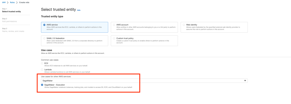
Click Next and click Next on the Add Permission screen (note the AmazonSageMakerFullAccess should be added by default. We will come back and add the required permission for S3 bucket access. Name your role and click ‘create role’.

We will need add the additional permissions for S3 access via an inline policy. The roles screen search for your role created above and open it up.

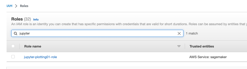
Open up your role and click on ‘Add permissions’ then click on ‘Create inline policy’

Click on the JSON tab and over write the existing code with the code below and update the field ‘your-bucketname-here’ field with your bucket name in both places.

{
  "Version": "2012-10-17",
  "Statement": [
    {
      "Action": [
      "s3:ListBucket"
      ],
      "Effect": "Allow",
      "Resource": [
        "arn:aws:s3:::your-bucketname-here"
      ]
    },
    {
      "Action": [
      "s3:GetObject",
      "s3:PutObject",
      "s3:DeleteObject"
      ],
      "Effect": "Allow",
      "Resource": [
        "arn:aws:s3:::your-bucketname-here/*"
      ]
    }
  ]
}

Click ‘Review Policy’, name your policy and click ‘Create Policy’.

Jupyter notebooks are found under Amazon Sagemaker. Open up the Amazon Sagemaker service window and expand Notebooks on the left hand side menu. Click on Notebook instances. Click the orange button labeled “Create Notebook Instance”. Essentially the ‘Notebook instance’ is an EC2 instance running the Jupyter software.

Name your notebook, select Notebook instance type ml.t3.medium (this should be default) , Select Platform identifier as Amazon Linux 2, Juptyer Lab 3. In the role drop down, select the IAM role you created in the previous steps. Click ‘Create notebook Instance’. Your instance will start to deploy and move from pending status to InService status when ready. Click on the name of your Notebook Instance. Then click on the ‘Open Jupyter’ button and you should with the standard Jupyter server GUI. On the Right hand Side of you screen click on the New button and select ‘conda_python3‘ kernel.

At the top of screen double click on ‘Untitled’ and change name to something more appropriate plot-tutorial01, and click the rename button.

In the git repository there is file notebook cells.txt with the text we will use in to generate our simple line plot.

In Jupyter cells you use the shift key plus the enter key together to run the code in the cell. The text in blue to left of the cell In [ ] will display an asterisks * to indicate that the code is running eg In [ * ] .

AWS notebooks include several libraries such as numpy, panadas and matplotlib by default. We just need to import them into your notebooks via the import command. In the fist cell we will import matplotlib library with the command then press shift enter

from matplotlib import pyplot as plt

In the screenshot above note the asterisk (*) in indicating the cell code ins being executed. During the cell execution you may get a message ‘

Matplotlib is building the font cache; this may take a moment.

Ok lets enter in our data manually first time around to keep this simple. Add the following code into cell block which represents chocolate bars costs over the several years. Note, this is completely fictitious data for demonstration purposes only.

bar_year = [2015, 2016, 2017, 2018, 2019, 2020, 2021, 2022]
bar_snickers = [110, 113, 114, 116, 120, 120, 123, 135]
bar_mars = [100, 105, 107, 118, 122, 124, 127, 140]
bar_bounty = [106, 108, 110, 113, 117, 118, 121, 128]

OK lets start building our plot. We will add each series and the order we add to plt object will determine the layering of the plot. We will use the plt object we imported in the first cell. Once you execute the code a default plot is generated.

That was pretty easy to get the default graph generated. However to make the graph useful it will need a title, labels, etc. Update last code block with:

plt.plot(bar_year, bar_snickers, label='Snickers')
plt.plot(bar_year, bar_mars, label='Mars')
plt.plot(bar_year, bar_bounty, label='Bounty')
plt.title('Chocolate bar manufacturing cost ')
plt.xlabel('Year')
plt.ylabel('Manufacturing cost / cents')
plt.legend()
plt.show()

If you are interested in building your own unique style you take plots up a level be specifying line colours and markers use try the following code change.

plt.plot(bar_year, bar_snickers, color='#DC143C', linestyle='-', marker='v', linewidth=3, label='Snickers')
plt.plot(bar_year, bar_mars, color='#CCA43D', linestyle='--', marker='s', linewidth=3, label='Mars')
plt.plot(bar_year, bar_bounty, color='#7AD7F0', linestyle=':',marker='o', linewidth=3, label='Bounty')
plt.title('Chocolate bar manufacturing cost ')
plt.xlabel('Year')
plt.ylabel('Manufacturing cost / cents')
plt.grid()
plt.legend()
plt.show()

The Matplotlib ‘fmt’ web page has details of line styles, marker available for use.

There a number of built in plot styles. You can display these with the following command:

plt.style.available

One of the available styles available is ‘ ggplot’ to use this style add the following:

plt.style.use('ggplot')

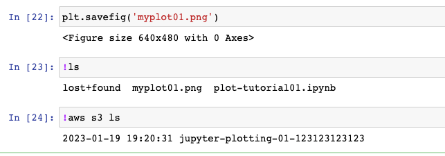
To save your plot use (where myplot01.png is the filename)

plt.savefig('myplot01.png')

To access Bash and Bash utilities such as the AWS CLI we need to prefix !. The list local files we use

!ls

To discover list of S3 bucket you have list access, run the following command:

!aws s3 ls

To save files to persistent storage (ie your S3 bucket) run the following command:

!aws s3 cp myplot01.png s3://jupyter-plotting-01-123123123123
!aws s3 cp plot-tutorial01.ipynb s3://jupyter-plotting-01-123123123123

Finally don’t forget to stop or delete your notebook instance to avoid ongoing costs.